After you read this essay, you will be able to use Bayesian reasoning on your own problem — and read the advanced books without fear.
You have seen the Bayes theorem in school. You may have opened a professional toolbox such as PyMC it bounced you off.
You suspect that you are missing something, but you cannot name it.
You might even be a professional in the field, using the formulas like reflexes and only hoping that a different explanation would make your work that much simpler.
This essay names it.
School presents the Bayes update rule like this:
\[p(A|B) = \frac{p(B|A)\,p(A)}{p(B)}\]
The equation is correct. It is easy to prove. And yet, when you face a real problem, it does not tell you what to do. Even professional data scientists get stuck here. The equation fails us in practice for two reasons.
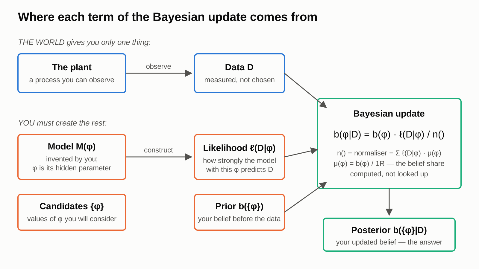
Reason 1: the notation hides where each term comes from. All four terms are written with the same letter \(p\), as if they were the same kind of thing. They are not:
In paper-and-pencil mathematics, symbols are shortened to save hand movements. Computer science learned long ago that such savings are counter-productive. We will un-shorten them.
Reason 2 — the important one: the equation says nothing about the model of the world. School trains us to expect that the we are given an equation that describes the world, and with some simple transformations, it’s all we need. The teacher said \(F = ma\), and every exercise follows from it.
Bayes does not work like that. The Bayes rule tells you nothing about how the world works. Before the rule can tell you anything, you must create a model of the world yourself — and construct its likelihood function. Only then can Bayes tell you how good each version of your model is. No amount of staring at the update equation produces the likelihood function; it is just not in there.
This is a common missing link.
Books often spend time on discussing the priors at length — informative, uninformative, how to defend yours — but the update is useless until you understand where the likelihood function comes from. And it’s the creation of the model that should be discussed.
And the answer is: you invent it.
To keep the concepts tied to reality, we start with a plant. A plant is a word, used to describe any object or process with inputs and outputs — a coin, a sensor, a market, a patient. The plant produces data \(D\), which we can observe.
We describe the plant with a model \(M\).
There can be more than one good model for the same plant; this topic alone deserves a book. However, let’s just take this for granted now, and press on.
Let’s say that the model (that you have just invented) takes a hidden (latent) parameter \(\phi\), so that, loosely, \(D = M(\phi)\). We cannot measure \(\phi\) directly. We can only observe \(D\) and hold beliefs about \(\phi\).
One more grounding point, often confused: in Bayesian reasoning, nothing on your desk is random. The likelihood values, the prior, the posterior — all are deterministic computations. The only place where randomness can live is inside the plant, and your model of the plant has to describe how this randomness produces data \(D\) as a function of \(\phi\).
It is hence very important to keep the distinction between these three things.
The three are measured on the same 0-to-1 scale, which is probably why history gave them the same letter \(p\).
To strengthen the distinction between types of measures the Bayes rules expects, we can attach units to the values:
| Unit | Concept | Example reading |
|---|---|---|
| \([R]\) | belief | 0.7 R: “I am 70% sure this value of \(\phi\) is the true one.” |
| \([\Omega]\) | probability | 0.8 Ω: “the model assigns probability 0.8 to what the instrument recorded.” |
A unit tags the type of a number. Every \([\Omega]\)-value in this essay is computed by the model of the plant: once you have invented the model, it produces these numbers; you never set them by hand.
The sample fraction needs no unit of its own: it never appears in the update rule, and that absence is the point — data reaches belief only through the likelihood.
Let’s give each concept its own letter and let the letter state the term’s job.
(We write the script letter \(\ell\), not plain \(l\), because plain \(l\) is too easy to confuse with \(1\), \(I\), and \(|\). Where \(\ell\) cannot be rendered, write \(L\) — the capital is also standard for likelihood in statistics.)
With these letters, the update rule reads:
\[b(\phi|D) \leftarrow b(\phi) \times \frac{\ell(D|\phi)}{n()}\]
Every symbol now has one meaning, and the equation itself shows the flow: posterior = prior scaled by how well this candidate \(\phi\) explains the data.
But wait! Yes we have a usable Bayes update formula with no ambiguities, but we still need the model of the plant, AND the likelihood function \(\ell()\).
As for constructing, or choosing, the model of the plant, it is truly beyond the scope of this essay.
Let me explain however how to construct the likelihood function \(\ell()\).
We will do the classic method: a bit of theory first, then some worked examples to follow.
To prime your brain, the worked example models will be:
import numpy.random
rng = numpy.random.default_rng(seed=42)
y = rng.binomial(1, phi, size=1)# note: this is a starter function, we will have to extend it and we will learn why
import numpy
x = numpy.array([...])
y = x * phi_propThe word likelihood sounds close to probability, and it drags in the wrong instincts. Here is a reading that keeps the types straight: the likelihood is like betting on the outcome and the likelihood function is the function that produces this bet.
It so happens that, over many rounds of play, the winning strategy is to place your bets on the outcomes at precisely their true probabilities. Any persistent deviation bleeds your money away — and the further your bets are from the truth, the faster the bleed.
The update rule then reads as settling the bets: the Bayes factor \(\ell(D|\phi)\,/\,n()\) compares each candidate’s stake with the belief-weighted average stake, and belief flows towards the candidates that bet on what happened more strongly than expected.
(This reading is old and respectable — de Finetti built the whole subject on bets; see the references page.)
Better asked: what should I believe about the bias of this coin?
For simplicity, and before getting into vectors and distributions, let’s ask a small question: we suspect that the coin could have one of 3 biases: \(0.2\), \(0.5\), or \(0.8\). How to quantify our belief about which is the most likely?
The plant is a coin. Our model \(M\): each toss gives 1 with probability \(\phi\) and 0 with probability \(1-\phi\). A fair coin has \(\phi = 0.5\); if there was a \(\phi = 0.1\) it would mean a coin that is heavily biased towards zeros. The model ignores the coin landing on its edge : models are allowed to approximate.
We want the likelihood function to reflect the probability of each outcome, assuming that the coin has a bias of \(\phi\).
Hence, probability of “1” is \(\phi\) and probability of “0” is \(1-\phi\) :
\[\ell(D{\equiv}1\,|\,\phi) = \phi \qquad \ell(D{\equiv}0\,|\,\phi) = 1-\phi\]
This function did not come from the Bayes rule and it did not come from the world. We built it from our model. We invented it, just here.
This step — not the update that follows — is where the real work of Bayesian reasoning happens.
We consider three candidate values for phi: \(\{\phi\} = [0.2, 0.5, 0.8]\) ;
We start with an “uninformative” prior, \(b(\{\phi\}) = [\tfrac13, \tfrac13, \tfrac13]\).
In other words, we want to see what Bayesian reasoning tells us we should change about our starter belief that the coin is unbiased.
We toss twice and get \(D = [0, 0]\). Independent tosses are settled independently, so each candidate’s stakes multiply: candidate \(\phi = 0.2\) staked \(0.8\) on each zero, and \(0.8 \times 0.8 = 0.64\); candidate \(\phi = 0.8\) staked only \(0.2\) each time, and \(0.2 \times 0.2 = 0.04\). Then:
prior = Q([1/3, 1/3, 1/3], R)                      # beliefs carry R
likelihood = coin_likelihood([0, 0], phi_grid)     # [0.64, 0.25, 0.04] Ω
posterior = belief_update(prior, likelihood)       # [0.69, 0.27, 0.04] R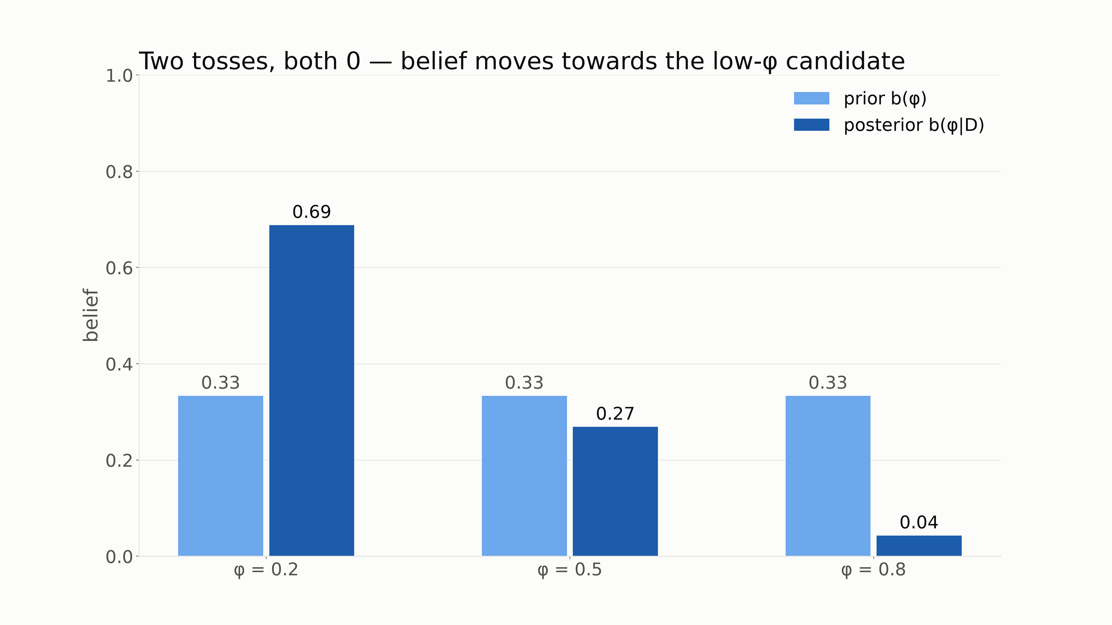
Two zeros in a row shift belief strongly towards the low-bias candidate — but the “unbiased hypothesis” of \(\phi = 0.5\) keeps a healthy 27%. Two tosses are weak evidence, and the posterior says so, quantitatively.
I will leave the exercise of looking how different priors affect the posterior to the reader.
Feed tosses one at a time, using each posterior as the next prior:
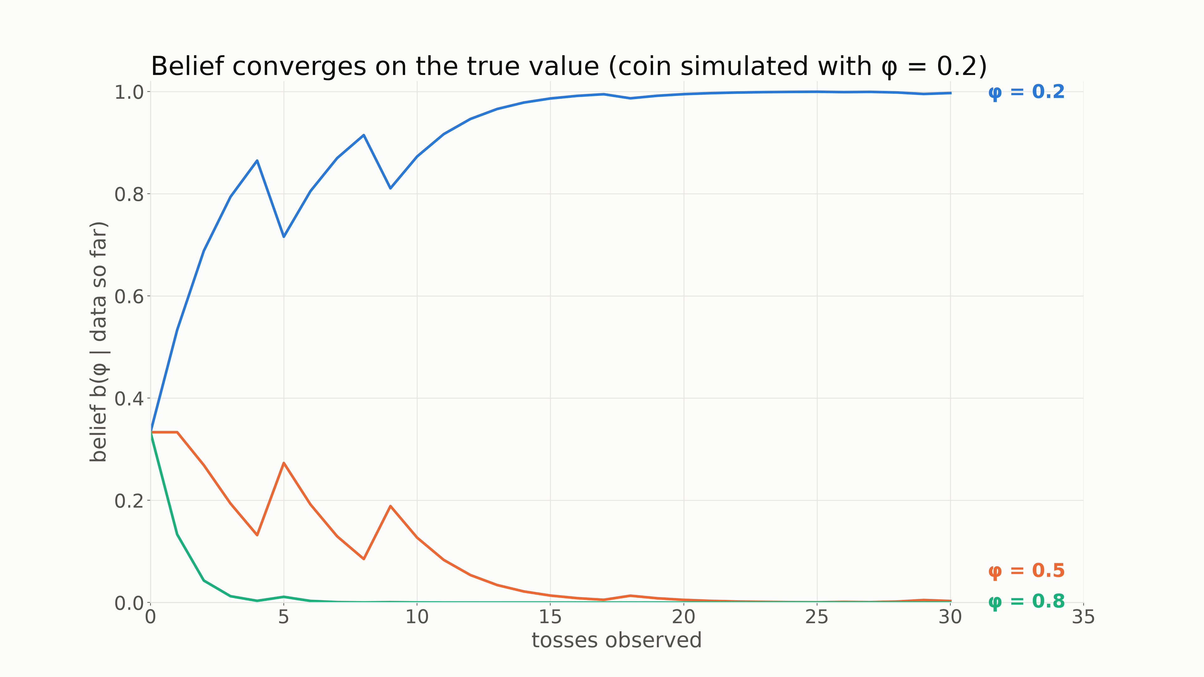
If the coin was in fact \(\phi = 0.2\) (in the real world, we cannot know that – we can only infer from the data), by thirty tosses the belief in \(\phi = 0.2\) is close to 1, and the wrong candidates are extinguished.
Note the dips: single contrary observations move belief the wrong way, and further data recovers it. That is not a flaw; that is what honest reasoning under uncertainty looks like.
Run it yourself:
pixi run python examples/coin_toss.py
pixi run python examples/make_figures.pyBoth coin updates above divided by \(n()\) without ever opening it. Time to open it.
Classic texts call this term the “marginal probability” or the “evidence”. They still write it as \(p(D)\), as if it were a probability carried by the data alone — and thereby cause maximal confusion. It cannot be: the value needs a sum over all \(\{\phi\}\), with your beliefs as the weights. In programming terms, its type differs from the other \(p\)’s: those are plain numbers you can pass around, while this one is a function — a computation that must ingest an entire likelihood function and an entire prior before it can hand you back a number.
The honest, full signature is:
\[n() = n(D,\ \ell(),\ \{\phi\},\ w(\{\phi\})) = \sum_{\alpha \in \{\phi\}} \ell(D|\alpha)\, w(\alpha)\]
where \(\alpha \in \{\phi\}\) means “for each candidate \(\phi\) from the set \(\{\phi\}\), take one, temporarily name it \(\alpha\) and use that one only”
Note that the prior enters through its weight \(w() = b()\,/\,1\mathrm{R}\), not as raw belief \(b\) — the reason becomes visible in the unit check below.
The sum runs over a fresh symbol \(\alpha\), so it does not collide with the single \(\phi\) in the update rule. (In the classic notation, the \(\phi\) inside the sum silently means “all \(\phi\)s” while the \(\phi\) outside means “this one \(\phi\)” — a notation conflict that breaks ordinary substitution rules.)
Also, note that this function takes a function \(\ell()\) as a parameter (!). and this is where many books cause confusion again, by plugging in their custom “model of the world” too early.
\(n()\) is your model’s prediction of the data. Read the sum as one weighted average: every candidate states how probable the recorded data is, and the prior decides how much each candidate gets to vote. The result is the probability that you — your model and your beliefs, acting together — assigned to \(D\) before you looked.
So it is a prediction about the world, but one issued from your desk, not measured off the plant. (The likelihood is no different in kind: you invented the model, so none of these numbers come from the world; that was the point of the previous sections.) What singles \(n()\) out is narrower, and more useful: it is the one place in the update where your beliefs enter as ingredients, not merely as the thing being updated.
If the word “evidence” ever bewildered you here, blame the English, not the mathematics. Evidence sounds like something found at the crime scene, identical for everyone who looks. But the data were the evidence; \(p(D)\) never measured the data — it measures your surprise at the data. And surprise is belief-relative by construction: the same instrument record that shatters one researcher’s worldview is precisely what another predicted all along. Two reasoners with different priors will compute different values of \(n()\) for the same \(D\), and both are right — each computed their own surprise.
Within the update rule, this number’s only job is bookkeeping: divide by the expected stake so the posterior sums to 1. (Outside the update rule, the same number gets a second life: a model that repeatedly assigns high \(n()\) to what actually happens is a model that saw the world coming — the basis of Bayesian model comparison. Not needed today.) The classic \(p(D)\) masks all of this behind a letter that looks like the other three — a symbol that lists the data as its only input, while silently summing over your whole grid at your own weights. That is why this essay gives it its own letter and its own name: the normaliser.
Or shorter: \(n()\) was never the world’s surprise at anything. It was always yours.
The full, substitution-safe update rule is:
\[b(\phi|D) \leftarrow b(\phi) \times \frac{\ell(D|\phi)}{\sum_{\alpha \in \{\phi\}} \ell(D|\alpha)\, w(\alpha)}\]
We gave belief and probability their own units. Units obey two rules, the same rules as in physics:
Both symbols of the prior already obey these rules. \(w() = b()\,/\,1\mathrm{R}\) is itself a rule-1 operation: \([R]/[R]\) cancels, in the open, and out comes a plain number. Dividing by \(1\,\mathrm{R}\) means “divide by your total belief budget” — so \(w()\) is the weight of belief on a candidate, and the weights always sum to 1.
Now push the units through the whole update and watch every step balance.
Read the formula as what it is: a weighted average of the likelihood, with weights \(w\):
\[n() = \sum_{\alpha \in \{\phi\}} \ell(D|\alpha)\,w(\alpha) = \mathbb{E}_{w}\!\left[\,\ell\,\right]\]
In words: the probability you expected the data to have, before you saw it — which is what the classic texts meant by “the evidence”. Expectations have carried units correctly for three hundred years, always the same way: the averaged quantity keeps its unit, the weights are dimensionless. Compute the average height of a population, \(\bar{x} = \sum_i x_i f_i\): the \(x_i\) are in metres, the population fractions \(f_i\) are plain numbers, and the average of metres is metres. Same here: an average of \([\Omega]\)-quantities is an \([\Omega]\)-quantity. Each term of the sum carries \([\Omega \cdot 1] = [\Omega]\), all terms match, rule 2 permits the sum, and \(n()\) carries \([\Omega]\). (Continuous data changes nothing here: with the measurement cell, each \(\ell\) value is already a true probability.)
The Bayes factor \(\ell(D|\phi)\,/\,n()\) is \([\Omega]/[\Omega]\) — a ratio: “how much better than expected did this candidate predict the data”. The posterior is \(b(\phi) \times \text{(pure number)}\), which carries \([R]\). Belief in, belief out. No step breaks; no symbol carries two meanings.
If you had written raw \(b\) inside the normaliser’s sum instead of \(w\), the units would refuse: each term would carry \([\Omega \cdot R]\), and the posterior would come out with no unit at all. That refusal is the unit system working — it rejects the mis-parse that treats an expectation’s weights as if they were the quantity itself. The \(w\) symbol makes the wrong version unwritable.
The unit bookkeeping now derives three facts that we earlier only asserted:
Units-Rule 2 also rejects a whole family of classic mistakes before they produce a wrong number:
The toolbox enforces all of this (
bayesian_reasoning/units.py, built onsympy.physics.units). Beliefs are taggedQ(values, R), likelihoods come back tagged withOMEGA, and a forbidden operation raises aUnitErrorthat states the rule and hints at the correct next step. A likelihood built from a density earns itsOMEGAstamp throughas_probability(density × cell), which refuses to stamp anything that has not cancelled to a plain number. The conversion from belief to weight is one explicit, visible call:prior.weight(), implementing literally \(w() = b()\,/\,1\mathrm{R}\).
That’s all of what I wanted to say, really. At this point, you are
ready to tackle any Bayesian reasoning problem. I would recommend you go
see the excellent statistical rethinking series by Richard
McElreath at youtube: statistical
rethinking playlist ; it starts slow but I promise the content is
excellent throughout.
If however, you want to hear more about the reasoning on how to construct the likelihood function in practice, continue here.
The coin had two outcomes and one parameter. Now take a proposition about continuous data — weight grows in proportion to height, \(y = x \cdot \phi_{prop}\) — and build its model three times. Each stage changes exactly one thing, and each stage teaches one lesson about constructing \(\ell()\).
Three people step on the scale. The scale records to 0.1 kg:
| person | height \(x\) [m] | weight \(y\) [kg] |
|---|---|---|
| 1 | 1.70 | 76.5 |
| 2 | 1.60 | 74.3 |
| 3 | 1.85 | 81.2 |
We consider three candidate coefficients, \(\{\phi_{prop}\} = [30, 45, 60]\) kg/m, with an uninformative prior, as before.
Start with the boldest model on the table — no noise at all:
\[y = x \cdot \phi_{prop}\]
This model predicts one exact weight for every height. In betting
language: each candidate places its entire stake of 1 on a single record
— the cell of the scale that contains its prediction. The likelihood
function is therefore one comparison; the stake was on the recorded
cell, or it was not (examples/linear_regression.py):
def certain_likelihood(x, y, prop_grid, cell=0.1):
    predicted = x.reshape(-1, 1) * prop_grid.reshape(1, -1)  # people in rows, candidates in columns
    hit = numpy.abs(predicted - y.reshape(-1, 1)) < cell / 2
    return as_probability(hit.astype(float).prod(axis=0))
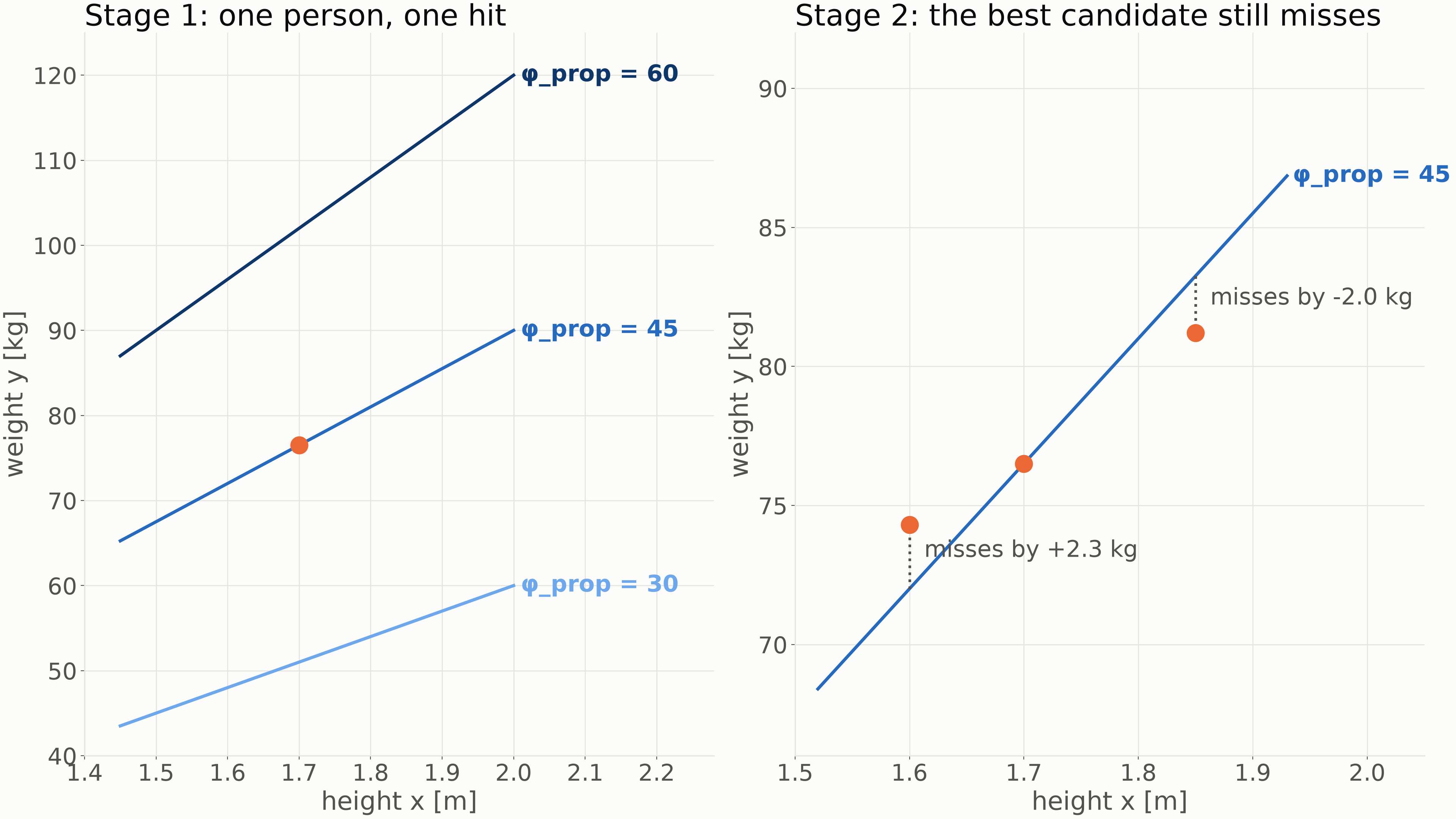
Feed it person 1 only. The candidates predict 51.0, 76.5 and 102.0 kg; the scale said 76.5. Likelihoods: \([0, 1, 0]\). Posterior: \([0, 1, 0]\) R.
One measurement, and belief collapsed to certainty. That is not a malfunction. A model that stakes everything on one outcome, and wins, deserves everything. (Full disclosure: we put \(45 = 76.5/1.70\) on the candidate list ourselves. A certain model whose grid misses the truth loses every candidate on the first observation — hold that thought; it is about to matter.)
Now feed all three people. Candidate 45 predicted \(1.60 \times 45 = 72.0\) kg for person 2; the scale said 74.3. A miss of 2.3 kg — nothing by bathroom-scale standards, but the model had bet everything on 72.0 and nothing on 74.3, so its stake on the recorded data is 0. The other candidates miss by more. Multiply each candidate’s stakes over the three people, and every product is 0.
Push \(\ell = [0, 0, 0]\) into the update, and the normaliser — the expected stake — is 0 as well. The toolbox refuses, and its error message is the lesson:
ValueError: normaliser must be positive: the model gave the data zero
probability under every candidate — no update is possible from this likelihood.
This is the ruin rule of betting: a candidate that staked 0 on what happened has posterior belief exactly 0 R, and no amount of later data can revive it. Here all three candidates are ruined at once, and the update has nothing left to renormalise.
Read the failure precisely, because the fix depends on it. The certain model is not wrong about the line — the figure shows candidate 45 passing beautifully close to all three people. It is wrong to bet everything on the line. Real weights scatter around any line — muscle, breakfast, shoes — and a model that assigns probability 0 to scatter has called the actual world impossible. The mistake is not in the update, and not in the prior. It is in the model. A likelihood function must spread its stake over everything the plant can actually do.
Admit the scatter into the model, as a noise term:
\[y = x \cdot \phi_{prop} + N(0, \phi_\sigma)\]
Two hidden parameters now: the coefficient \(\phi_{prop}\), and the scatter width \(\phi_\sigma\) — because honestly, we do not know the width of the scatter either. We will ask the update to learn both.
How does a model bet on a continuum? It cannot name every outcome one by one, so it spreads its stake by similarity: much on the cells near its predicted line, less further away. How fast the stake falls with distance is a modelling choice — ours says Gaussian. With the residual \(\Delta = y - x \cdot \phi_{prop}\), the familiar shape:
\[\ell(y\,|\,\phi_{prop}, \phi_\sigma) = \exp\!\left(-\frac{\Delta^2}{2\phi_\sigma^2}\right)\]
Large misses are heavily penalised but no record is impossible — the ruin of stage 2 cannot happen. Every value lands in \([0, 1]\), and the values across candidates need not sum to anything: the normaliser eats the scale.
A constructed likelihood can fail quietly — run it and look. Run the update with this likelihood over a 2D candidate grid and it recovers \(\phi_{prop}\) nicely — but the belief in \(\phi_\sigma\) runs to the largest candidate on the grid, every time. Why: a bigger \(\phi_\sigma\) forgives every miss more, and this function never charges for the forgiveness. As built, \(\phi_\sigma\) is unlearnable.
The charge it forgot is the budget. Every candidate’s bets over all possible records total exactly 1 — that is just its probabilities summing to 1 — so a stake spread over a wide range of outcomes must lie thin: a tolerant candidate can never win big on any single record. That is the price of tolerance. The bare exponential ignores the price: it lets every candidate, however wide, stake the full 1.0 at its own centre. The repair is the prefactor of the full Gaussian density:
\[\ell(y\,|\,\phi_{prop}, \phi_\sigma) = \frac{1}{\phi_\sigma\sqrt{2\pi}} \exp\!\left(-\frac{\Delta^2}{2\phi_\sigma^2}\right)\]
A wide \(\phi_\sigma\) now pays rent: it spreads its stake thinly, so a data point near the line rewards it less than a tight candidate. A tight candidate stakes high near its line and pays for it on outliers. With the prefactor in place, both parameters become learnable — the update can finally weigh confidence against tolerance.
One debt remains from the notation section, and it falls due exactly here. The prefactor at \(\phi_\sigma = 5\) kg is \(1/(5\sqrt{2\pi}) \approx 0.08\) per kilogram — and for a tight \(\phi_\sigma = 0.2\) kg it would be \(2.0\) per kilogram. Per kilogram? Textbooks shrug: “for continuous data the likelihood is a density, and a density can exceed 1” — and leave you to swallow that. The measurement cell dissolves it instead.
No real instrument records an exact real number. It records to a finite resolution \(\Delta D\): our scale showing 76.5 kg is really saying “inside the 0.1-kg-wide bin around 76.5”. So the recorded event has an honest probability: the model’s density (stake per kilogram) times the cell width \(\Delta D\) (kilograms) — the units cancel, and out comes a plain number in \([0, 1]\). A density of 2.0 per kg is not “a probability above 1”; it is a rate, waiting for a cell width to become a probability. One rule covers continuous and categorical alike: \(\ell\) is the model’s probability of what the instrument recorded — for a coin toss, the category is its own bin, and no \(\Delta D\) appears at all.
Three facts make \(\Delta D\) painless. It is a property of your instrument, never of the candidate \(\phi\). It is therefore identical for every candidate, so it cancels in the Bayes factor \(\ell/n\) — the posterior does not depend on it. And so you never need to know its value. (Stage 1 was the one exception that proves the rule: the certain model had no width of its own, so the instrument’s cell was the only width in the problem, and its value 0.1 kg appeared in the code. The moment the model owns a width \(\phi_\sigma\), the cell retreats to bookkeeping.)
The bookkeeping is worth automating, because it catches the trap of this whole stage mechanically. A density carries “per kg”, and the \(1/(\phi_\sigma\sqrt{2\pi})\) prefactor is what carries it; the bare exponential carries nothing. Multiply each by the cell:
joint_density = Q(per_obs.prod(axis=2), kg**(-n_obs))  # per kg^N
cell = Q(1.0, kg**n_obs)                               # the instrument's; its value cancels in ℓ/n
return as_probability(joint_density * cell)            # stamps Ω only if the units cancelled
With the prefactor, the kilograms cancel and
as_probability stamps the result \([\Omega]\). Without it, a stray kg survives
and the toolbox raises UnitError before a single wrong
belief is computed. The \(\phi_\sigma\)
trap is machine-caught.
(Two footnotes for the careful reader. Several observations multiply into a joint probability, which keeps the single tag \(\Omega\) — the tag marks a type, not a physical dimension, so it does not exponentiate. And textbook density notation is simply the \(\Delta D \to 0\) limit: every \(\ell\) shrinks by the same factor, ratios stay fixed — when Stan or PyMC report a log-posterior “defined up to an additive constant”, your cell width is part of that constant, harmless for exactly this reason.)
Three people are too few to pin down two parameters, so we let the simulated plant supply 25:
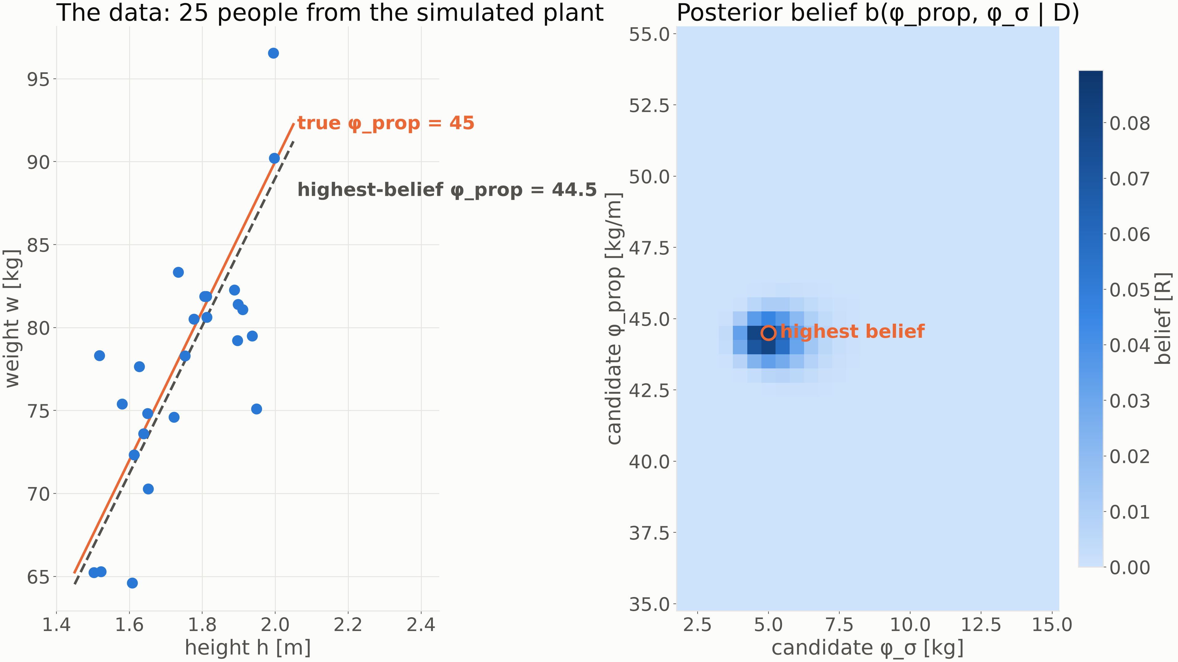
From 25 people (true \(\phi_{prop} =
45\), \(\phi_\sigma = 5\)), the
highest-belief candidate lands at \(\phi_{prop} = 44.5\), \(\phi_\sigma = 5.0\). Run it:
pixi run python examples/linear_regression.py. The toolbox
needed zero changes across all three stages — each
model brought its own likelihood function, and
belief_update never cared what the candidates meant.
This is a likelihood function, not the likelihood function. If your plant’s noise is not Gaussian, build a different one — the freedom to choose the model is not a bug in Bayesian reasoning; it is the whole point. But the three stages leave you a checklist: spread your stake over everything the plant can do (or one surprise ruins every candidate), make every candidate pay for its tolerance (or the wide ones freeload), and after you construct a likelihood, test that it can actually learn each parameter you care about.
Good — that is the correct prior. Contact me on LinkedIn and tell me why I am wrong.
The prior art that informed this notation is collected on the references page.
This essay is partially inspired by the exposition of importance of good notation, Tau Manifesto